Deep dive · Time series & forecasting
4th of 50+ teams · Data hackathonCan Google Searches See Inflation Before the BLS Does?
An alternative-data model for next-month CPI, and the audit that showed my own headline number was an illusion. AutoML reported RMSE 0.39 and R² 0.96. A one-line random walk scores 0.363. This is what was left after I took the leakage out.
2025 · IDSC machine learning competition · team of four · my scope: pipeline, modeling, validation
- Observations
- 188 months
- Coverage
- Jan 2010 - Aug 2025
- Search terms
- 13 → 3 signals
- Feature space
- 28 → 13 PCs (95% var)
- Backtest window
- 68 months, out of sample
- Placed
- 4th of 50+ data hackathon teams
The lag problem
Official CPI arrives two to three weeks after the month it describes. For anyone allocating capital or setting prices, that means reacting to a world that has already moved. Google search volume is available the same day, and when people start searching gas prices and rent, they are reacting to prices they have just paid.
The premise is clean: convert search volume into a leading indicator and buy back the lag. It placed 4th of 50+ teams at the Illinois Data Science Club's data hackathon. This write-up is about what happened when I went back afterwards and checked the result.
Getting the data to exist
Two sources, one of them hostile. FRED’s CPIAUCSL series is a clean API call. Google Trends is not: pytrends aggressively rate-limits, and a 13-keyword pull fails long before it finishes.
The fetch layer is built around that constraint: keywords requested one at a time, exponential backoff starting at 45 seconds and growing 1.5× per retry, five attempts each, and every successful response written to an on-disk cache keyed by keyword and timeframe. Once a term is cached the pipeline never re-requests it, which turns a run that fails halfway into a run that resumes. That cache is the only reason 15 years of data across 13 terms exists at all.
Eleven food keywords became one column
Individual grocery terms such as egg prices, milk price, bread price and beef prices were too noisy to use on their own, because each is dominated by its own commodity shock rather than by general food inflation. Rather than drop them, the pipeline z-scores all eleven and averages them into a single food_index_trend, then discards the components. The composite lands at r ≈ 0.27 with CPI YoY, modest but stable, where every individual term was not.
The merge is an inner join on month-end that drops months missing search data rather than interpolating across them, which would manufacture history that never happened. Final dataset: 188 complete months, no gaps.
The number that lied
PyCaret compared a dozen model families on the PCA features and ranked them by out-of-sample RMSE. A cluster of linear models (OLS, Ridge, Bayesian Ridge) came in at RMSE ≈ 0.39, R² ≈ 0.96, against a dummy baseline of 1.88. Tree ensembles were meaningfully worse. Bayesian Ridge won on robustness to multicollinearity.
An R² of 0.96 on a macroeconomic forecast should be alarming. Central banks with hundreds of economists cannot forecast CPI that well. So before writing it up, I ran the one check that settles it: how well does “next month will look like this month” do?
0.363. The random walk beats the winning model. Everything the pipeline had learned, it had learned from CPI’s own inertia, and it had not even learned that as well as copying the last value. Three compounding defects produced the illusion.
The answer was in the feature set
PCA received 28 features. Thirteen were CPI’s own history: the level, MoM, YoY, and lags 1/2/3/6/12 of both. The leakage guard excluded any column named future_, which blocked the target but nothing else. CPI YoY moves roughly 0.36pp per month, so a model handed today’s YoY and asked for next month’s has been handed the answer. PCA rotates that information; it does not remove it.
Nine features were observations from the future
The “lead” features are built with shift(-k). gas_prices_trend_lead3 at month t holds search volume from t+3, two months after the value being predicted. Nine such columns entered the model. They cannot exist at prediction time, which makes any model that uses them undeployable regardless of its score.
The validation split ignored time
train_size=0.8 with fold_shuffle=True produces random folds over a monthly series whose adjacent observations are near-duplicates. The model trained on the inflation surge before being tested on it. Chronological splits are not a stylistic preference for time series; they are the only split that answers the question being asked.
The fix
Rebuild the evaluation so the model only sees what it would have had on the morning of the forecast: strictly lagged features, a chronological split at January 2019, and a random-walk baseline printed next to every score it produces. The number gets much worse and much more useful.
| Metric | Search model | Random walk | Seasonal |
|---|---|---|---|
| RMSE | 2.831 | 0.469 | 3.040 |
| MAE | 2.232 | 0.348 | 2.377 |
| Directional accuracy | 55.9% | 69.1% | 33.8% |
Why it lost
The model was fit on a decade in which inflation never exceeded 3.81% and had a standard deviation of 0.90. It was then asked about a period that reached 9.00%.
3.81%
highest CPI YoY in training, 2010-2018
9.00%
peak CPI YoY in the test window, Jun 2022
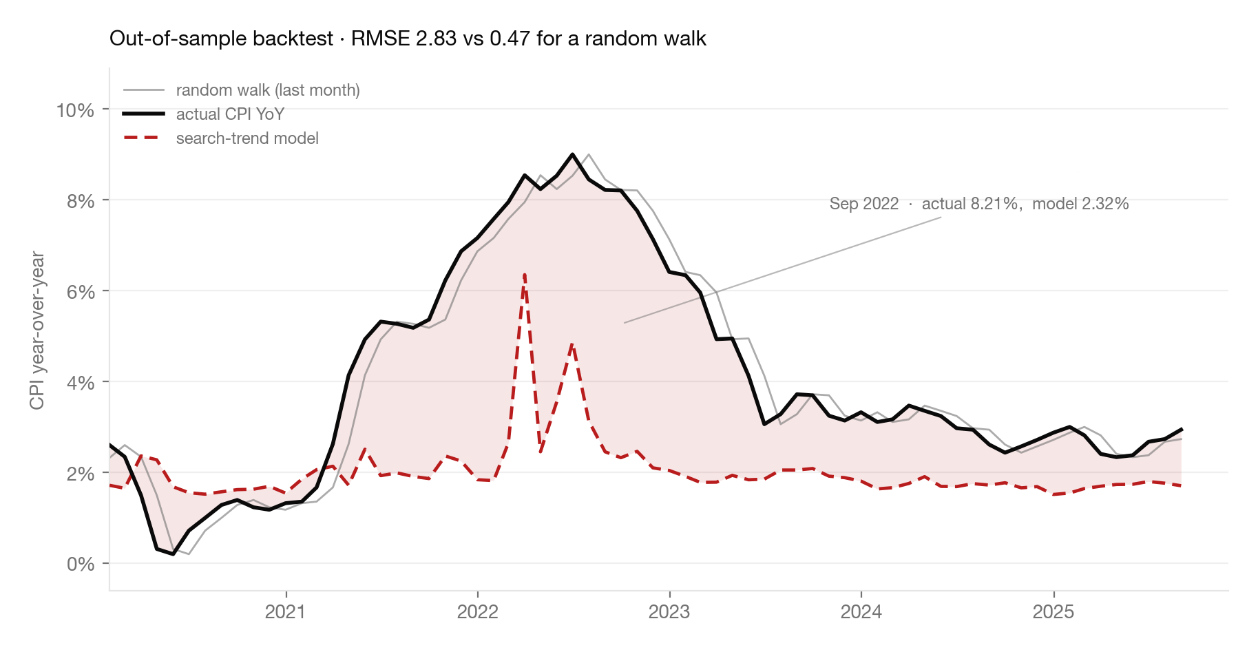
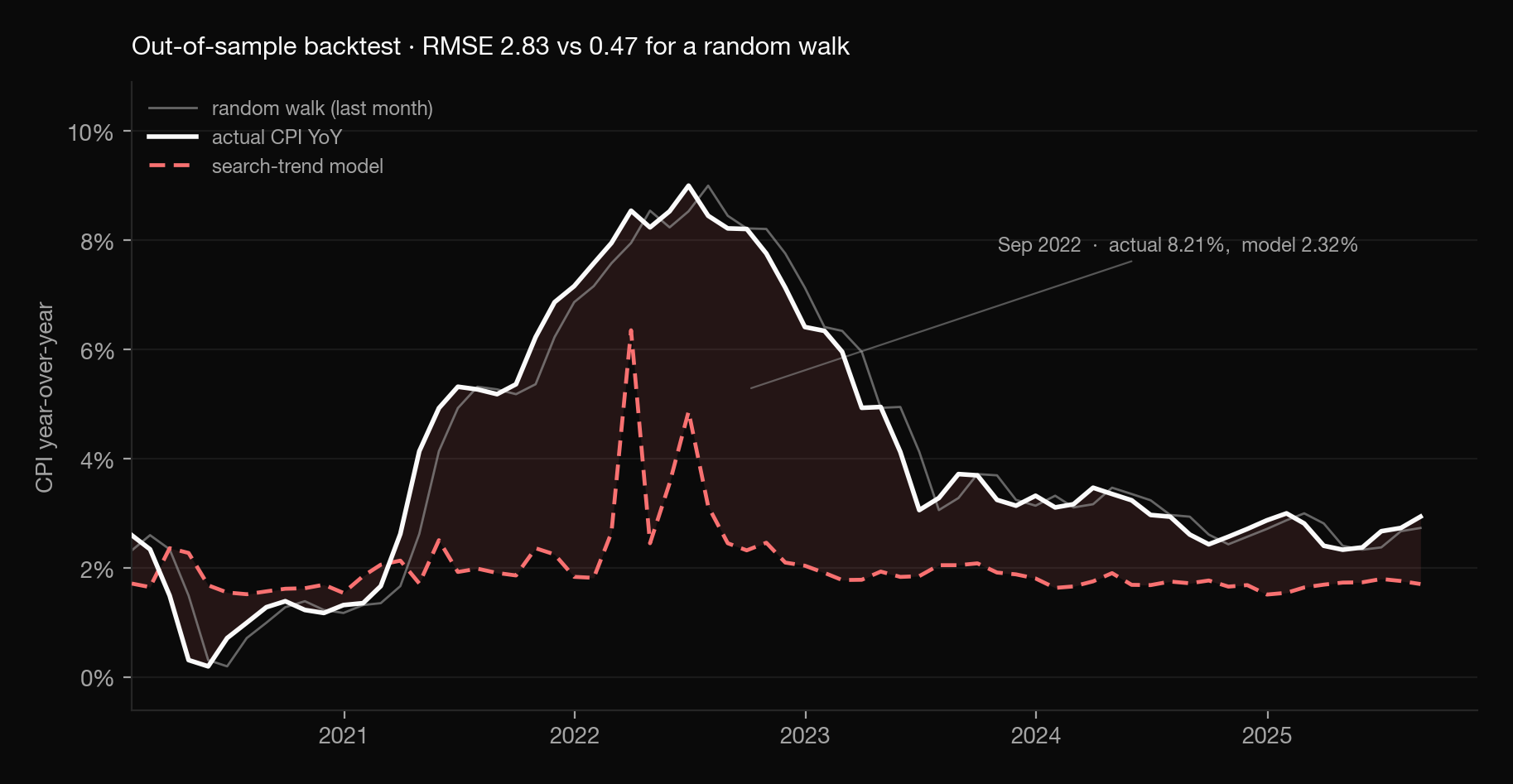
Across all 68 test months the largest value the model ever produced was 6.35%. In September 2022, with actual CPI YoY at 8.21%, it predicted 2.32%, a 5.9-point miss. Broken out by regime the pattern is unambiguous: RMSE of 0.90 through 2019-20, 4.24 through the 2021-22 surge, and 1.80 as inflation normalized. The model is competent in the regime it was trained on and blind outside it.
This is the finding I would defend hardest. A linear model fit on a quiet sample does not fail gracefully when the world changes state; it fails silently, and it fails most at exactly the moment anyone would want to rely on it. No amount of feature engineering fixes that, because it is a property of the training distribution.
What the search data is actually worth
Rent leads. Gas does not.
Correlation with CPI YoY at increasing lead k, in months:
| Search term | k=0 | k=1 | k=2 | k=3 |
|---|---|---|---|---|
| rent | 0.205 | 0.240 | 0.265 | 0.285 |
| gas prices | 0.560 | 0.544 | 0.538 | 0.543 |
| food index | 0.267 | 0.264 | 0.273 | 0.262 |
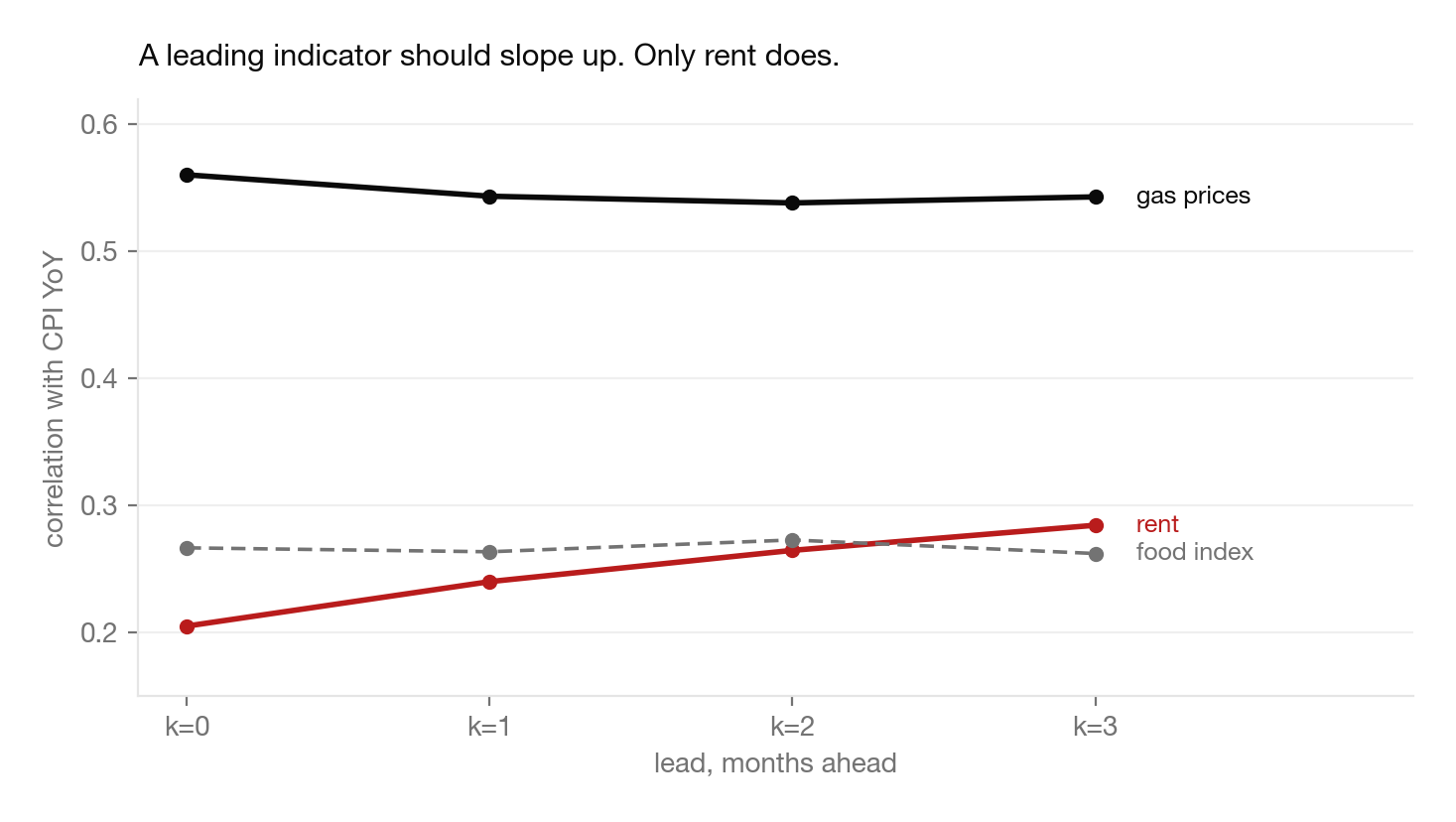
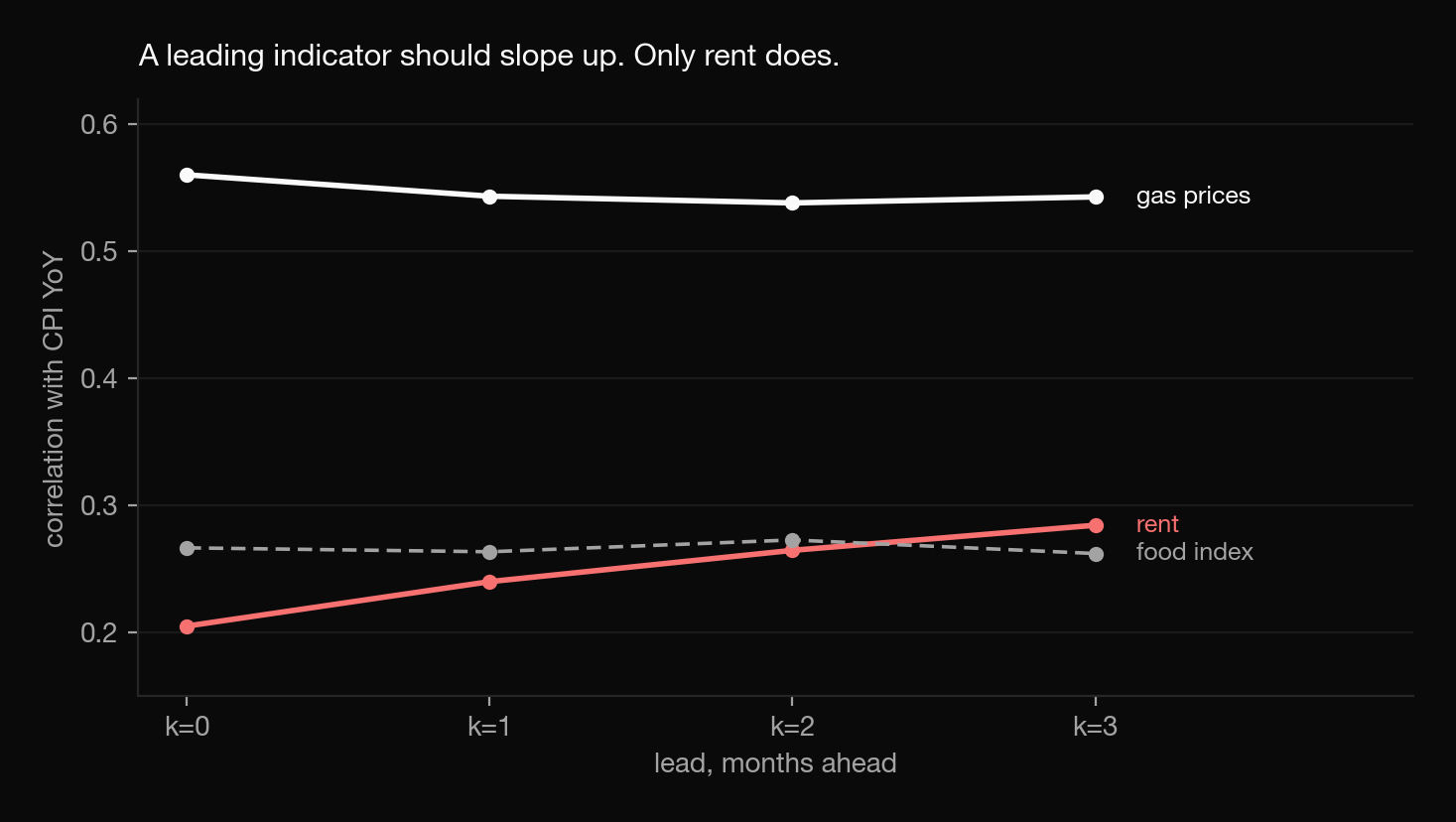
Rent rising with lead is a genuine lead-lag signature, and one with a mechanism behind it: leases reprice annually, so search interest builds months before the change reaches the index. Gas is the mirror image, strongest at zero lead and flat thereafter. Gas searches are a nowcasting input, not an early warning. Our deck claimed a 1-2 month window for policymakers; the correlation structure only supports that for rent.
One caveat I hold myself to: rent searches carry a strong annual cycle. Part of that rising profile may be seasonal alignment rather than economic lead, and separating the two requires deseasonalizing first.
The signal only works when inflation is news
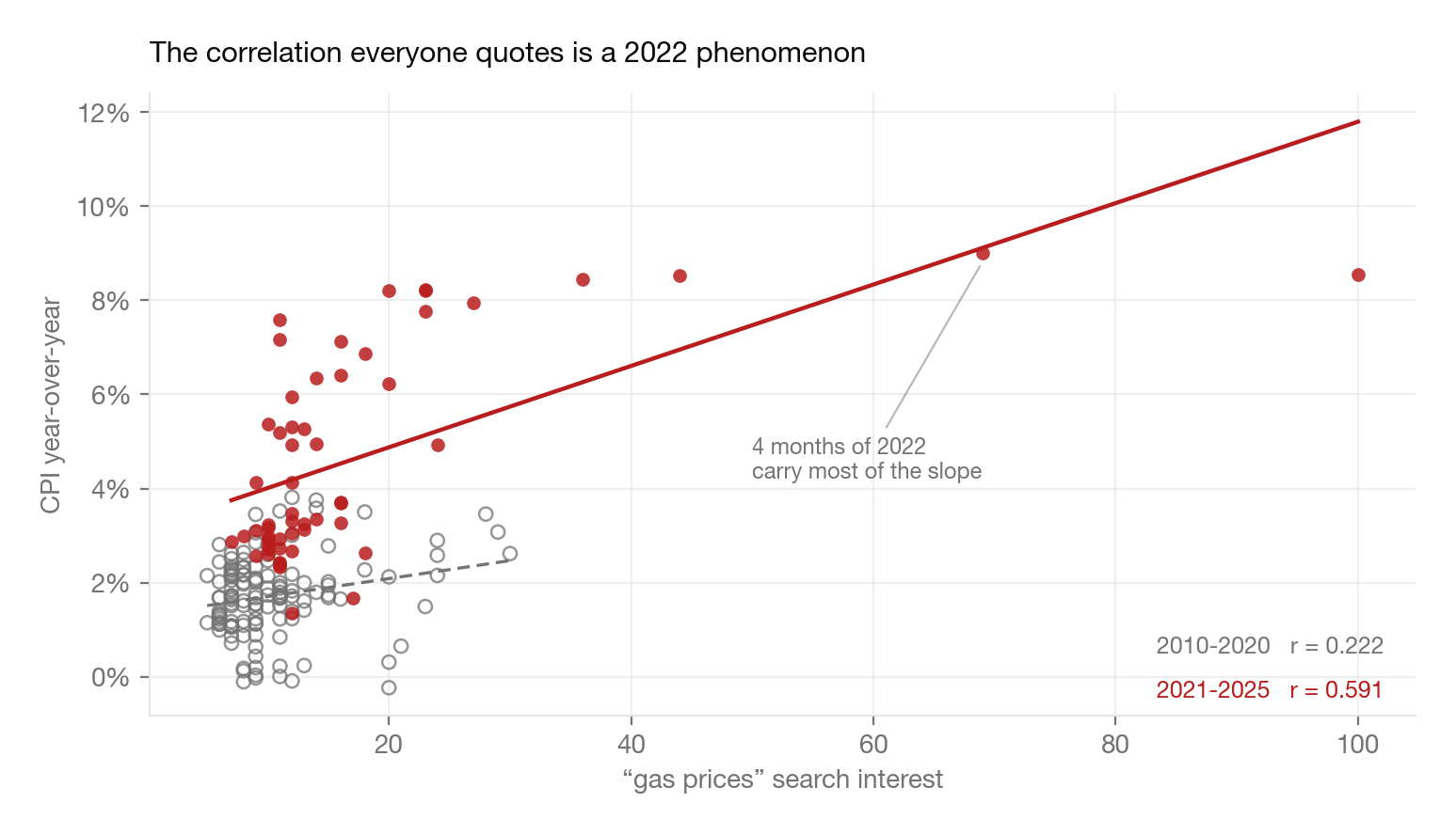
The 0.560 headline correlation is not a stable property of the relationship. Across 2010-2020 it is 0.222. From 2021 onward it is 0.591. Drop the five months where the gas search index exceeded 30, four of them in 2022, and the full-sample figure falls from 0.560 to 0.457. Spearman’s rank correlation, which ignores outlier magnitude entirely, is 0.460.
The finding
The relationship is real, and it is state-dependent. Search behavior tracks inflation precisely when inflation is salient enough for people to search about it, and carries almost nothing when it is not. That means a search-based early-warning system is least informative during the calm periods when an early warning would be worth the most.
A last measurement to size the ceiling: PCA on the three search series alone, with no CPI history at all, produces a chronological-holdout RMSE of 2.06 against a target standard deviation of 1.92, worse than predicting the mean. On its own, search data cannot forecast the level of inflation. Whatever value it has is in direction, and conditional on regime.
What I would build next
- 01
Score against the random walk, not against zero. Skill relative to persistence should be the headline metric. A model that cannot beat “nothing changed” has not earned a number.
- 02
Predict the change, not the level. Targeting ΔYoY, or the residual from the random walk, removes the autocorrelation the model was hiding behind and forces the search features to carry their own weight.
- 03
Walk-forward re-fitting. An expanding window that re-estimates every month would let coefficients adapt as a regime shifts, instead of freezing 2018’s understanding of inflation for the next seven years.
- 04
Quantile or robust regression. Least squares on a calm sample produces a model that structurally cannot output a surge. Quantile regression at least admits the tail exists.
- 05
Weekly EIA gasoline prices. Higher-frequency ground truth for the strongest signal, and a way to test the lead structure at weekly rather than monthly resolution.